SAP HANA Cloud Machine Learning Challenge: Preventing Employee Churn

Dirk Kemper

Jan 1, 2023 8 min read Enterprise AI

In December 2022 SAP held a machine learning competition called “I quit!” attended by 50 participants to showcase the machine learning capabilities of SAP HANA Cloud. The idea is to predict from a database of employees who is the most probable to be leaving his or her job in the short term, based on historical information of employees which have quit recently.

The idea of the challenge is not only to create a well-performing model to predict employee churn, but also to put this into a broader picture by providing a storyline of how this model could be integrated into an organization and who would be benefiting from this.

The dataset for this challenge has been delivered by SAP and was accessible to all participants.

Storyline

Let’s say we are trying to develop an application for an HR department to see what we can do about preventing employee churn. The goal is that we would like to get insights into the reasons employees may be quitting in the future and to find out what measures the company may be taking to prevent this.

Can we create a predictive model that not only tells which employees will be quitting their jobs but also why this was the case and how to prevent this?

Let’s find out!

Machine learning approach

Predicting employee churn is a fairly classical machine learning problem which belongs to a broader class of problems called binary classification. The task of the machine learning algorithm is to predict for each employee whether there is a risk of the employee churning (i.e. quitting) or not. Hence the name binary, as it needs to predict one out of two classes.

HANA Cloud has a range of machine learning algorithms available in both the APL and PAL libraries. APL is more focused on business users who would like to get quick results whereas the PAL library is suitable for data scientist, allowing for more fine-grained control over the machine learning algorithms.

I personally like the APL because of the short time to value: you just supply it a dataset to have APL handle cumbersome tasks like train/test set splitting, variable discretization, analysis of multicollinearity and variable importance. Nowadays the APL has a gradient boosting tree classifier under the hood which is still one of the most capable algorithms for solving these kinds of tabular data problems.

As stated the classification algorithms available in the PAL allow for more fine-grained control over the modeling process, with the added cost of more manual data preprocessing and hyperparameter tuning but could have been applied just as well for this problem.

For the training and analysis purposes I will be using a Jupyter notebook as this is the de facto standard for data science and machine learning activities nowadays. You will notice how straightforward it is to access the in-database machine learning functionality in HANA from the Jupyter notebook by using SAP’s hana_ml library.

To view the full output of the analysis please have a look at the following Jupyter notebook: https://github.com/kemperd/sap-hana-ml-challenge/blob/master/Training_and_analysis.ipynb

If you want to follow along yourself, take the data from https://github.com/kemperd/sap-hana-ml-challenge/blob/master/Emp_Churn_Train.csv and upload this into a HANA database in a table called EMP_CHURN.

First I will split up the data into a training and holdout set. Note that the APL will perform its own splitting of the train set into training and validation sets which are used by the algorithm internally for its own optimization. The holdout set will not be fed to the algorithm and will serve as a true test set that I will use for validating performance after the training.

train, test, valid = train_test_val_split(emp_churn_all, testing_percentage=0.2, validation_size=0)

The data will be stored into their own tables:

train.save('EMP_CHURN_TRAIN', force=True)
test.save('EMP_CHURN_TEST', force=True)

Now lets fit a gradient boosting tree using the APL as follows:

model = GradientBoostingBinaryClassifier(variable_auto_selection = True)

model.set_params(
    extra_applyout_settings={
        'APL/ApplyExtraMode': 'Advanced Apply Settings',
        'APL/ApplyPredictedValue': 'true',
        'APL/ApplyProbability': 'true',       
        'APL/ApplyDecision': 'true',   
    })

model.fit(train, label='FLIGHT_RISK', key='EMPLOYEE_ID')

Note that I have asked the APL to output a few advanced apply settings which are useful to get more insights into the details of the predictions and to learn why the algorithm is making specific choices.

Now apply the dataset onto the data in the test set table:

apply_out = model.predict(test)
pdf_apply_out = apply_out.collect()

I will be using the Area Under Curve (AUC) metric for determining the quality of the classifier. This is the area under the ROC curve which can be obtained by looking at the true and false positive rates. This number will be in the interval [0..1] where we want it to be as high as possible. For some more details on this approach please see https://en.wikipedia.org/wiki/Receiver_operating_characteristic.

model.get_performance_metrics()['AUC']

The AUC is about 0.90, which indicates a sufficiently well performing classifier.

Now let’s examine what features of the dataset appear to be most important towards predicting the target:

model.get_feature_importances()

The top-5 features are:

FUNCTIONALAREACHANGETYPE (24%)
PROMOTION_WITHIN_LAST_3_YEARS (14%)
TIMEINPREVPOSITIONMONTH (9%)
EMPLOYMENT_TYPE_2 (8%)
AGE (3%)

These are summing up to 58%, while the other features make up for the remaining 42%.

This means that the functional area change type is the most important. Lets see what this field contains:

emp_churn_all.agg([('count', 'FUNCTIONALAREACHANGETYPE', 'COUNT')], group_by='FUNCTIONALAREACHANGETYPE').collect()

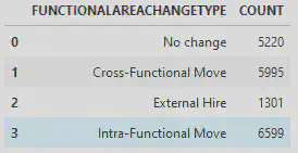
The field seems to be an indicator whether an employee has recently moved between functions, across functions or whether it is an external employee. We will use this later on to see if we can modify this employee status to prevent them from churning.

First we will have a look at the predictions to count the number of employees that the model predicts may be churning soon:

emp_flightrisk = apply_out.filter('PREDICTED = \'Yes\'')
num_flightrisk = emp_flightrisk.describe('EMPLOYEE_ID').collect()['count'].values[0]
print('Number of employees in test set with positive flight risk: {}'.format(num_flightrisk))

This gives an amount of 468 employees which the model predicts are about to quit.

Now we will join the employee numbers as given by the prediction back with the original dataset to retrieve all data for those churning employees:

emp_flightrisk_new = emp_flightrisk.alias('L').join(emp_churn_all.alias('R'), 'L.EMPLOYEE_ID = R.EMPLOYEE_ID', select=[
    ('L.EMPLOYEE_ID', 'EMPLOYEE_ID'),
    'AGE', 'AGE_GROUP10', 'AGE_GROUP5', 'GENERATION', 'CRITICAL_JOB_ROLE', 'RISK_OF_LOSS', 'IMPACT_OF_LOSS', 
    'FUTURE_LEADER', 'GENDER', 'MGR_EMP', 'MINORITY', 'TENURE_MONTHS', 'TENURE_INTERVAL_YEARS', 'TENURE_INTERVALL_DESC',
    'SALARY', 'EMPLOYMENT_TYPE', 'EMPLOYMENT_TYPE_2', 'HIGH_POTENTIAL', 'PREVIOUS_FUNCTIONAL_AREA', 'PREVIOUS_JOB_LEVEL', 
    'PREVIOUS_CAREER_PATH', 'PREVIOUS_PERFORMANCE_RATING', 'PREVIOUS_COUNTRY', 'PREVCOUNTRYLAT', 'PREVCOUNTRYLON', 
    'PREVIOUS_REGION', 'TIMEINPREVPOSITIONMONTH', 'CURRENT_FUNCTIONAL_AREA', 'CURRENT_JOB_LEVEL', 'CURRENT_CAREER_PATH',
    'CURRENT_PERFORMANCE_RATING', 'CURRENT_REGION', 'CURRENT_COUNTRY', 'CURCOUNTRYLAT', 'CURCOUNTRYLON', 
    'PROMOTION_WITHIN_LAST_3_YEARS', 'CHANGED_POSITION_WITHIN_LAST_2_YEARS', 'CHANGE_IN_PERFORMANCE_RATING',
    'FUNCTIONALAREACHANGETYPE', 'JOBLEVELCHANGETYPE', 'HEADS'
])

pdf_emp_flightrisk = emp_flightrisk_new.collect()

Note that the last statement is collecting the data in a Pandas DataFrame to perform some local modifications within the Jupyter notebook.

These are the counts per distinct value for the FUNCTIONALAREACHANGETYPE field for the churning employees:

pdf_emp_flightrisk['FUNCTIONALAREACHANGETYPE'].value_counts()

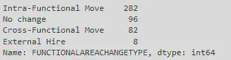
We will remove the external hires from the dataset, as the company cannot influence their function in the same way as internal employees:

pdf_emp_flightrisk.drop( pdf_emp_flightrisk[(pdf_emp_flightrisk['FUNCTIONALAREACHANGETYPE'] == 'External Hire')].index, inplace=True)

For the remaining employees, their FUNCTIONALAREACHANGETYPE will be set to ‘Cross-Functional Move’ to see what the effect is:

pdf_emp_flightrisk['FUNCTIONALAREACHANGETYPE'] = 'Cross-Functional Move'

The Pandas DataFrame will be stored back into HANA table CHURNING_EMPLOYEES as follows:

create_dataframe_from_pandas(conn, pdf_emp_flightrisk, 'CHURNING_EMPLOYEES', force=True)

At this point we have a table called ‘CHURNING_EMPLOYEES’ in HANA which contain all internal employees about to churn, with their FUNCTIONALAREACHANGETYPE statuses set to ‘Cross-Functional Move’. This table will be input into the apply algorithm again to once again retrieve the number of churning employees:

emp_churning = DataFrame(conn, 'select * from CHURNING_EMPLOYEES')
apply_out_new = model.predict(emp_churning)

Now let’s examine the effect:

emp_flightrisk_new_pos = apply_out_new.filter('PREDICTED = \'Yes\'')
num_flightrisk_new = emp_flightrisk_new_pos.describe('EMPLOYEE_ID').collect()['count'].values[0]
num_flightrisk_delta = num_flightrisk - num_flightrisk_new
print('Number of employees in test set with positive flight risk after change in Functional Area Change Type from No change to Cross-Functional Move: {}'.format(num_flightrisk_new))

print('This is down {}, which means that {:.1f}% of employees can possibly be prevented from churning by allowing them a Cross-Functional Move'.format(num_flightrisk_delta, num_flightrisk_delta / num_flightrisk * 100))

This outputs the following:

Number of employees in test set with positive flight risk after change in Functional Area Change Type from No change to Cross-Functional Move: 146 

This is down 322, which means that 68.8% of employees can possibly be prevented from churning by allowing them a Cross-Functional Move

This means that there are 322 less employees of the employees for which the model predicts they are about to churn that can possibly be retained by allowing them a Cross-Functional Move, which is 68.8% of the total!

This is a factor that the company can definitely influence and also means that employee churn should not be regarded as a naturally occurring phenomenon but can be guided in the direction that benefits the company.

Wrapup

This blog post has shown some great results in analyzing employee churn from a database. I have shown a predictive modeling approach that does not only tell us what employees may be about to be quitting, but also why this is the case and how they can be prevented from leaving the company!

By applying targeted measures towards the employees that are about to be quitting the model predicts it may be possible to reduce employee churn by 68.8%!

This functionality is readily accessible from any SAP HANA or HANA Cloud system and is straightforward to fit into a modern data science workflow using Jupyter notebooks and the hana_ml library.

HANA APL