Beyond Static Image Generation: Taking Stable Diffusion to the Next Level

In my last blog post I have shown how to download the Stable Diffusion model weights and set up an image generation workflow yourself using the Stable Diffusion model as provided by the Huggingface Transformers library. Although these text-to-image generation results can be pretty awesome, you can get similar results by interfacing with the DALL-E 2 playground which is publicly accessible without being on a wait list nowadays.

The key feature that sets Stable Diffusion apart from API-based image generation offered by DALL-E 2 is -again- the fact that the model weights can be downloaded to your own machine and be used to locally instantiate the neural network that comprises the image generation capabilities. Today I will show you how to leverage this to get some very interesting and creative results which are just as great.

The technique I will show is in this blog post is called a latent space exploration or a latent space walk. The first author I have seen put this into practice is Andrej Karpathy (former Tesla). The work I will present now is from Ian Stenbit and François Chollet, who you may know as the author of Keras and his fundamental book on deep learning in Python. You can read their post here: https://keras.io/examples/generative/random_walks_with_stable_diffusion/. This post will lean on their work but gives its own angle into describing what it going on under the hood.

In contrast to my previous article I will be using TensorFlow with Keras instead of PyTorch. Keras has a great implementation of Stable Diffusion available which is very easy to set up and tries to get an edge over PyTorch by emphasizing performance in two ways:

1. Keras provides a mixed-precision mode (i.e. float16 numbers) which helps on modern NVIDIA GPUs by utilizing the on-chip Tensor Cores
2. It is also able to use a so-called XLA-compiler which should help with speeding up TensorFlow models

Latent space

In order to understand what is meant by latent space, let’s investigate the Cambridge Dictionary definition of the term latent:

Present but needing particular conditions to become active, obvious or completely developed.

This sums up it up nicely. As I have shown in my previous post you can get quite different results by adding keywords to your prompts to steer the outcome. However, it is not fully clear what the full extent is of the images that the model is able to generate, as the prompting mechanism is opaque and driven by lots of trial and error. Therefore, many images are impossible or at least very difficult to be extracted from the model by simply providing text prompts, so therefore they are latent. In this post I will show you a few ways how you are able to extract those images after all.

The diffusion process

Let me try to give you an idea of how Stable Diffusion performs its image generation magic under the hood. From a high-level perspective, the main function of the algorithm is to convert a patch of random noise to an image for which you have provided the caption. To learn how this works, you should look at the way that the Stable Diffusion model you can download yourself has actually been trained.

Let’s say we are training the algorithm on a photo of a dog. We want the algorithm to learn the transition of the original photo to a patch of noise, in let’s say 50 steps.

1. The photo is converted into an array of 50 photos, linearly spaced out. Each step in the array is adding the same amount of noise to the photo, where the 50th photo is a full patch of noise.
2. Each photo is entered into the diffusion model, indicating it’s prompt (“photo of a dog”) and the step in the noise-addition process.
3. We want the algorithm to indicate the amount of noise added between the current and previous step. This is the reason why providing the step number is important.
4. The output of the model after each step is an image containing only the noise the model believes has been added to the image.
5. The process is iterated 50 times until the full patch of noise has been reached.

I hope you can see where this leads: if you now would reverse this process, i.e. give the model a somewhat noisy image (say at step 20) you can have the model denoise that image to its previous step.

You can now take this idea all the way to step 50 where you provide a fully random patch of noise, provide the caption (“photo of a dog”) and have the model denoise the random image in 50 iterations to get an image of your caption. And presto, you now know how Stable Diffusion works under the hood!

Now there are a few more moving parts to this as indicated in the architecture. As is the case with any Transformer-based algorithm there is an encoder and decoder in the mix. The encoder generates a word embedding vector by passing the string through a language model. The decoder is responsible for upscaling the result of the diffusion process into an image of the size you requested, like 512x512. Note that the diffusion model responsible for the denoising operates on images of size 64x64 only. You can see this process depicted in the below architecture.

Interpolation

The first technique I will show you is prompt interpolation. This will create a fluid transition from one image into another by leveraging the word embedding vectors created by the text encoder. You can view these word embeddings vectors as a numerical presentation of the sentence you have entered. In this case this vector is actually a matrix of size 77x768. Any string you enter will be translated to its own unique matrix by the text encoder you can see in the Stable Diffusion architecture.

To interpolate two prompts let’s define them as follows:

• v1: A photograph of a dog
• v2: A photograph of a cat

For simplicity let’s regard the word embeddings as simple 2D vectors called v1 and v2 as shown in the below image. A nice property of word embeddings is that they convert a text string to a numerical representation, which opens the possibility of performing calculations with these numbers. To interpolate the prompts a few intermediate vectors are created by linearly filling the distance between the two vectors in 3 steps. These newly created vectors are shown as dotted lines:

The interpolated vectors may or may not represent an actual text prompt, but this does not really matter as their primary use is to input them into the diffusion model which will generate images that have a certain amount of similarity to either the image generated by v1 or by v2. Now we are actually exploring the latent space: the interpolated vectors refer to images which we do not know how to extract from the model by text prompts, but by using the properties of the word embeddings vector we now have a way to extract these images.

This example only shows 3 interpolated vectors, but obviously the transition between the prompts will be much more fluid if you use more vectors.

Note that in the real world this concept will be translated into interpolating two matrices of size 77x768, not just two 2D vectors.

Image interpolation example

I have used the following packages dependencies for running the code:

keras-cv==0.3.4
tensorflow==2.9.2
tensorflow_datasets==4.7.0
pillow==9.2.0

Note that the TensorFlow import is not the latest at this time of writing but this version did not give me CUDA-related problems that the latest version seemed to have.

First import the dependencies:

import keras_cv
from tensorflow import keras
import matplotlib.pyplot as plt
import tensorflow as tf
import numpy as np
import math
from PIL import Image

# Enable mixed precision
# (only do this if you have a recent NVIDIA GPU)
keras.mixed_precision.set_global_policy("mixed_float16")

# Instantiate the Stable Diffusion model
model = keras_cv.models.StableDiffusion(jit_compile=True)

The following function will be used to store all interpolated images in an animated GIF:

def export_as_gif(filename, images, frames_per_second=10, rubber_band=False):
    if rubber_band:
        images += images[2:-1][::-1]
    images[0].save(
        filename,
        save_all=True,
        append_images=images[1:],
        duration=1000 // frames_per_second,
        loop=0,
    )

Now generate the interpolated images from two text prompts:

seed = 12345
noise = tf.random.normal((512 // 8, 512 // 8, 4), seed=seed)

prompt_1 = "A photograph of a dog"
prompt_2 = "A photograph of a cat"
interpolation_steps = 150
batch_size = 3
batches = interpolation_steps // batch_size

encoding_1 = tf.squeeze(model.encode_text(prompt_1))
encoding_2 = tf.squeeze(model.encode_text(prompt_2))

interpolated_encodings = tf.linspace(encoding_1, encoding_2, interpolation_steps)

batched_encodings = tf.split(interpolated_encodings, batches)

images = []
for batch in range(batches):
    images += [
        Image.fromarray(img)
        for img in model.generate_image(
            batched_encodings[batch],
            batch_size=batch_size,
            num_steps=25,
            diffusion_noise=noise,
        )
    ]

export_as_gif("dog-to-cat.gif", images, rubber_band=True)

This will give the following result:

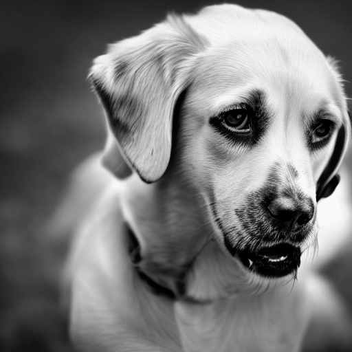
Let’s see another interesting result. It appears that the image interpolation works very well for fairly static scenes or scenes that are not too far apart in meaning. I will now show the results for the following prompts:

• prompt_1 = “A black and white photograph of a young boy’s face”
• prompt_2 = “A black and white photograph of an old man’s face”

Random walks

The next topic I will explore is the concept of a random walk. Similar to the prompt interpolation from the previous topic, here too the word embeddings vector is transformed for generating similar images. Let’s say we want to generate an image from the following prompt: “a photograph of an owl sitting on a tree branch”. This prompt will be represented by a vector called v1.

The idea is to “walk” away from the initial vector by iteratively taking the same small step in each dimension. When translated into a 2D vector this may look somewhat as follows:

The idea is that at each step the prompt will be ever so slightly different from the original, until it reaches a point where the prompt just represents noise. This way you can see the image evolving from an image exactly matching the original description to images which loosely resemble the prompt but do adhere to the original concept.

For this I will be using the following Python code:

walk_steps = 150
batch_size = 3
batches = walk_steps // batch_size
step_size = 0.002

encoding = tf.squeeze(
    model.encode_text("A photograph of an owl sitting on a tree branch")
)
# Note that (77, 768) is the shape of the text encoding.
delta = tf.ones_like(encoding) * step_size

walked_encodings = []
for step_index in range(walk_steps):
    walked_encodings.append(encoding)
    encoding += delta
walked_encodings = tf.stack(walked_encodings)
batched_encodings = tf.split(walked_encodings, batches)

images = []
for batch in range(batches):
    images += [
        Image.fromarray(img)
        for img in model.generate_image(
            batched_encodings[batch],
            batch_size=batch_size,
            num_steps=25,
            diffusion_noise=noise,
        )
    ]

export_as_gif("owl.gif", images, rubber_band=True)

The above code walking in 150 steps with a step size of 0.002 from the original image gives the following result:

You can see some interesting things happening here:

• The background of the photo fades and transitions into dots and later balls
• The photo of the owl evolves into a painted owl with its original position on the left side if the image
• The painted owl moves to the center of the image and transitions between painting styes
• The owl dissolves into vague owl-like dark shapes until only noise is left in the image

You can imagine these steps to be the reverse of the diffusion process, i.e. the target image is converted into its original noise.

Circular walk

The last example I will show is that of a circular walk. This is very similar to the random walk scenario, but instead of a straight line from the origin we will be walking a circle around the coordinate targeted by the text prompt. For a 2D vector this may look as shown below. The original vector is depicted as v1 while the dots around it are the result of the circular walk:

An interesting property of the circular walk is that the image will transition away from the original while in the end returning back to it. This can be accomplished by the following Python code:

prompt = "Skyline of New York City"
encoding = tf.squeeze(model.encode_text(prompt))
walk_steps = 450
batch_size = 3
batches = walk_steps // batch_size

walk_noise_x = tf.random.normal(noise.shape, dtype=tf.float64)
walk_noise_y = tf.random.normal(noise.shape, dtype=tf.float64)

walk_scale_x = tf.cos(tf.linspace(0, 2, walk_steps) * math.pi)
walk_scale_y = tf.sin(tf.linspace(0, 2, walk_steps) * math.pi)
noise_x = tf.tensordot(walk_scale_x, walk_noise_x, axes=0)
noise_y = tf.tensordot(walk_scale_y, walk_noise_y, axes=0)
noise = tf.add(noise_x, noise_y)
batched_noise = tf.split(noise, batches)

images = []
for batch in range(batches):
    images += [
        Image.fromarray(img)
        for img in model.generate_image(
            encoding,
            batch_size=batch_size,
            num_steps=25,
            diffusion_noise=batched_noise[batch],
        )
    ]

export_as_gif("circular-walk.gif", images)

As you can see I am using 450 steps for the simple prompt “Skyline of New York City”. This number of steps will increase the generation time quite a bit but allow for very detailed insights into the many images the model is able to generate, giving a mesmerizing effect.

Wrapup

In this post I have shown you how to move from simply prompting Stable Diffusion to generate static images to creating interesting smoothly transitioning animations. The main idea behind this is the concept of the latent space which can be very hard to reach by manual prompting but can be explored by using the numerical word embeddings vectors (or matrices in this case).

It is obvious that Stable Diffusion has a huge amount of visual information hidden inside its model which we can extract by other ways than providing it text prompts.